Charged Plates and more

Introduction

Some time has passed since my last update on this topic, and there are more new exciting features to implement. This chapter will mainly focus on implementing charged plates.

So, what is actually the current problem? The problem right now is that I only have static point charges which exert the electric fields, however, to act as a demonstration for class, I also now need to make charged plates. As of right now, the simulation follows a simplified pipeline where we contain the information about all the point charges and for every pixel, in the compute shader, we calculate the electric potential using $\varphi =k{q}_1/r$. As we sum up the potentials for every charge in relation to a single point, we store that info in a buffer and send it onto a different shader. This second compute shader, then, calculates the electric field using $\vec{E}=-\vec{\nabla }\varphi$ and also stores it inside a buffer. This electric field buffer is then directly used for the visualisations of the grid, and the movement of particles.

Adding metal plates into this pipeline seems simple, just alter the electric potential at the point where plate resides and et voilà! Unfortunately, not everything is that simple. Metal plates are not simple point charges, they have boundaries, and electrons and their own field inside the plate…

In this chapter we will try two approaches. First, the obvious one: treat the plate as a fixed potential and let the grid relax to approximate the answer — the Jacobi method. The method works, however is far too slow, so we will replace it with the Boundary ELement Method, which only solves for the charge on the plate’s surface.

General Solution

How do we go about dealing with this then? Well, let’s recap some conductor knowledge. A conductor, usually a metal plate, is full of ‘free’ electrons. If an electric field were to be exerted on the conductor, these electrons will perceive a force and start accelerating due to $\vec{F}=q\vec{E}$. In general, these electrons can either be moving, or be static. For the purpose of electrostatics, we will consider only the latter. This means that inside the conductor itself, the electric potential will be constant. Since the electric field is defined as the negative gradient of the potential, a constant potential gives $\vec{E}=-\vec{\nabla }\varphi =0$ inside the conductor. This also means that all of the conductor is an equipotential surface. By Gauss’s law we know that $\vec{\nabla }\cdot \vec{E}=\rho /{ϵ}_0$, so $\vec{E}=0$ inside means there is no charge inside the conductor. So how does a metal plate be charged at all? Well, the real answer is that the actual charge resides only on the surface of the conductor. The charges repel each other and want to get as far apart as possible, but they cannot leve the metal, so they end uup on the surface.

Now that we have recapped how conductors and metal plates work, lets think about what and how to change our simulation. Since our electric field $\vec{E}$ directly correlates to the potential, that is what we will be altering. In addition to the already existing sum of potential from charges we will now consider new regions. These regions will be passed in as a set of coordinates, defining the metal conductor boundary. This now means that for any point $(x,y)$ on the screen, we will have to first determine if its inside, outside or on the boundary with the region. If the point is inside, we set the potential to be a constant value, like $10V$.

Strictly speaking, forcing the whole interior to a constant is a modelling choice, we only guarantee the right potential on the boundary, and assume that the inside will follow same convention.

For any point on the boundary or outside the metal plate, only on initialisation, we set the potential to be zero. Afterwards, we can imagine blurring out the edges of this box, where with every compute pass the edges become more and more smeared out, creating that correct potential look. To account for these new regions we will have to make a ping-pong model of the potential buffer, since we will have to read, adjust values and write back.

Mathematical Derivation

We know Maxwell’s first equation to be

$$\vec{\nabla }\cdot \vec{E}=\frac{\rho }{{ϵ}_0}$$

Since we also know that $\vec{E}=-\vec{\nabla }\varphi$, we can combine the two forming

$$\vec{\nabla }\cdot (-\vec{\nabla }\varphi )=\frac{\rho }{{ϵ}_0}$$

by expanding $\nabla$ and the dot product within, we can make the following steps

$$\begin{array}{rl}\vec{\nabla }\cdot (-\vec{\nabla }\varphi )& =\frac{\rho }{{ϵ}_0}\\ ⟨\frac{\partial }{\partial x},\frac{\partial }{\partial y},\frac{\partial }{\partial z}⟩\cdot ⟨\frac{-\partial \varphi }{\partial x},\frac{-\partial \varphi }{\partial y},\frac{-\partial \varphi }{\partial z}⟩& =\frac{\rho }{{ϵ}_0}\\ \frac{-{\partial }^2\varphi }{\partial x^2}+\frac{-{\partial }^2\varphi }{\partial y^2}+\frac{-{\partial }^2\varphi }{\partial z^2}& =\frac{\rho }{{ϵ}_0}\\ \frac{{\partial }^2\varphi }{\partial x^2}+\frac{{\partial }^2\varphi }{\partial y^2}+\frac{{\partial }^2\varphi }{\partial z^2}& =-\frac{\rho }{{ϵ}_0}\\ {\nabla }^2\varphi & =-\frac{\rho }{{ϵ}_0}\end{array}$$

The ${\nabla }^2$ is called the Laplacian operator, which is — important to note — not a vector. In simple terms, this operator measures the difference between the value of $\varphi$ at a point and the average value of $\varphi$ in an infinitesimal circle around that point. Now, in any region without charges, $\rho =0$. This is the space around the plate, where we get the Laplace equation:

$${\nabla }^2\varphi =0$$

The plate itself acts as a boundary condition; we force $\varphi$ to a fixed value on it. This is called a Dirichlet boundary condition.

Note that we derived this term in 3D, however, our simulation only has $x$ and $y$, so the $\frac{{\partial }^2\varphi }{\partial z^2}$ term is dropped. Also, in this simulation every charge, and plate segment produces a potential in the form $kq/r$, as if the screen were a slice of a 3D world. The grid-based ‘blur’ below solves the true 2D equation, whos point-charge potential decays differently, so it can never actually match the analytic charges. This one more reason why — spoiler alert — we will eventually move away from it.

This gives us the final equation, which is best approximated using the previously mentioned ‘blur’. This so called ‘blur’ is achieved by simply getting the average of the 4 neighbours

Implementation

Now that we have defined the general setup and solution of the problem, we can start working our way towards solving it.

Data Input & Passing

Let’s think first about the how our data will be defined, processed and passed around. For a metal conductor we can define the coordinates of the four vertices, along with the charge on its surface:

struct Plate {
    // We will go in anti-clockwise direction starting at the bottom-left,
    // e.g. [0.0, 20.0, 10.0, 20.0, 50.0, 60.0, -10.0, 50.0] will give us:
    //
    // D(-10.0, 50.0) ---- C(50.0, 60.0)
    // |                   |
    // |                   |
    // |                   |
    // |                   |
    // |                   |
    // A(0.0, 20.0) ------ B(10.0, 20.0)
    //
    vertices: [f32; 8],
    potential: f32
}

Along with our static charges, we will also store a Vec<Plate>; it will have to be passed along with other constants to the all the shaders.

Now, consider a point $P(x,y)$ — how do we know it’s inside or outside the boundary defined by the 4 vertices? We can use a great analogy of us taking a train around the boundary of our surface. For every edge, we can use a simplification of a 2D cross product with points test point $P$, and line connecting $A$ and $B$ — $\left[(B_x-A_x)(P_y-A_y)-(B_y-A_y)(P_x-A_x)\right]$ — to find out if the point is on the left side (positive) or on the right side (negative). If the point is inside our shape, as we go along all of our edges, we will find that the direction is always the same, either always positive, or always negative. If one of the values ends up being zero, that means the point is on the boundary itself.

Currently, we have a single potential field which we pass to the shaders. Instead, we will have to create 2 separate buffers called A and B which will be juggled around in a ‘ping-pong’ model to continuously change the data. As one buffer is read from, the other is written to, then they swap positions. This allows us to re-use a single shader and a single layout by just altering which buffers we assign to the binding.

Shader Changes

Now that we have defined what type of data we will store and how we will pass it to the shader, lets talk about how the shader should be changed. Currently, our electric_potential_cs compute shader uses an analytic method to calculate the potential at any point in space. Instead, we will have to reserve to using the equations mentioned above. First, we loop through every plate that we have in our system and extract its vertices. These vertices (Vec2), along with our position on the screen, are fed into the function is_inside which returns an enum telling is if that point is inside, or outside our boundary. If the point was inside, we immediately set the potential to the one specified in the plate itself and return:

for plate_idx in 0..constants.num_plates {
    let plate = plates[plate_idx as usize];
    let edges = [
        Vec2::new(plate.edges[0], plate.edges[1]),
        Vec2::new(plate.edges[2], plate.edges[3]),
        Vec2::new(plate.edges[4], plate.edges[5]),
        Vec2::new(plate.edges[6], plate.edges[7]),
    ];
 
    match is_inside(current_coords, edges) {
        Condition::Inside | Condition::Boundary => {
            output[center] = plate.potential * constants.electric_options.charge_strength_scale;
            return;
        }
        _ => (),
    }
}

Now that we know that every point after this block of code will be a point outside of the conductor, we can use the previously mentioned ‘blurring’ method. This is done by taking samples of the potential around our center position, and averaging them out.

$$\begin{array}{ccccc}& & \boxed{(x,y+1)}& & \\ & & \updownarrow & & \\ \boxed{(x-1,y)}& \leftrightarrow & \boxed{(x,y)}& \leftrightarrow & \boxed{(x+1,y)}\\ & & \updownarrow & & \\ & & \boxed{(x,y-1)}& & \end{array}$$

This means that if we sample $\varphi$ at every position and then compute

$$\frac{{\varphi }_{\text{left}}+{\varphi }_{\text{right}}+{\varphi }_{\text{up}}+{\varphi }_{\text{down}}}{4}={\varphi }_{\text{avg}}$$

Why does averaging work tho? Approximating the Laplacian using the method of finite differences, will yeild us

$${\vec{\nabla }}^2\varphi \approx \frac{{\varphi }_{\text{left}}+{\varphi }_{\text{right}}+{\varphi }_{\text{up}}+{\varphi }_{\text{down}}-4{\varphi }_{\text{center}}}{h^2}$$

Setting this to zero and solving for ${\varphi }_{\text{center}}$ gives exactly the average of the four neighbours. However, adding back the fixed point charges is not as simple as adding on the potential to the average. We have to look back at our equation for empty space:

$${\nabla }^2\varphi =0$$

However, our space is not empty anymore! We have to obey the Poisson’s equation now, which we derived earlier:

$${\nabla }^2\varphi =-\frac{\rho }{{ϵ}_0}$$

This means that we have to calculate the charge density $\rho$ for all of our sources. Afterwards by combining and re-arranging we arrive at:

$${\varphi }_{\text{center}}={\varphi }_{\text{avg}}+\frac{h^2\rho }{4{ϵ}_0}$$

To actually calculate the charge density, we loop through every point charge and calculate the distance between that charge and our current position. Then, if that distance is smaller than the radius of the particle itself, we add the charge scaled by $1-\text{distance}/\text{radius}$, so it fades linearly from full strength at center to zero at edge of particle.

for charge_idx in 0..constants.num_charges {
    let charge = charges[charge_idx as usize];
    let charge_pos = charge.position;
    let charge_coords = Vec2::new(charge_pos[0], charge_pos[1]);
    let charge_charge = charge.charge * constants.electric_options.charge_strength_scale;
 
    let distance = (current_coords - charge_coords).length();
    // not really in PX's, so gotta play around with scaling this.
    let radius = constants.electric_options.charge_radius;
 
    if distance < radius {
        rho += charge_charge * (1.0 - distance / radius);
    }
}

Now, we can just sum the $\rho$ term to the neighbour average using the formula above and and write the result back, where after this compute call, the buffers A and B will swap and this process is repeated every frame. Now that we have the potential computed, a different shader will compute the electric field at any point and that will be used in our grid and more. However, when I have implemented tracing, I have decided to go with an analytical approach and directly re-computed the electrical field at any one point to calculate the direction of the field lines. This is not feasible anymore, hence that shader will have to be changed to fetch the electric field. This step and the vertex shader are omitted here, as they are standard boilerplate.

Problem with Jacobi Iteration

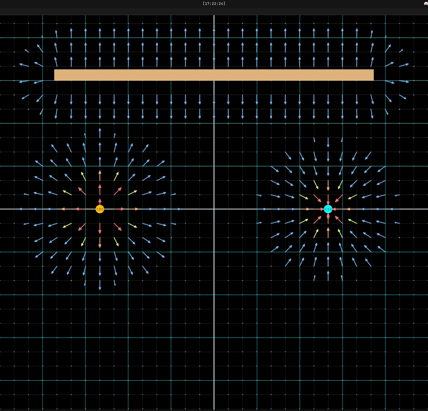
Now, if we have implemented our metal plates correctly, we can pass in our default value — which for now is a long metal plate directly above the two default charges — we should see a result on the screen.

But, there is a real issue here. One that I realised way too late. This is a dynamic simulation, meaning it takes time for information to propagate and the potentials to be computed. Before it was really simple, we had a single equation for any point on the screen, whereas now, we have basically a texture (or a buffer) which dynamically changes over time, and cannot be predicted. And if we leave it be as it is right now, it would take a couple minutes for the simulation to stabilise, and it does not look that pretty. However, I will note that it is quite amusing to see the simulation develop over time and for fields lines to converge to their locations, but highly impractical for our use. This can be combatted, short term, by increasing the number of compute passes done before sending off the data to the render pass.

let mut cpass = cmd_encoder.begin_compute_pass(&ComputePassDescriptor {
    label: Some("FirstComputePass"),
    timestamp_writes: None,
});
 
// Default: 64
for _ in 0..POTENTIAL_ITERATIONS {
    self.electric_pipeline.compute_potential(
        &mut cpass,
        &constant_bind_groups,
        &self.electric_manager.electric_bind_groups,
        self.electric_manager.size,
    );
}
drop(cpass);

Although this approach does help to reduce the time needed for electric fields to propagate, it is a heavy burden on the GPU and is still highly inefficient. To be more technical, what we have just implemented is Jacobi Iteration, where information propagates at a pace of 1 pixel per step. On an $N\times N$ grid, it takes on order of $N^2$ steps to settle and realx. Better grid solvers exist, but they are more complicated and out of the scope for the current chapter.

The Fix

Okay, so how do we go around this? Well, the method we chose initially was not so great, so we will have to find a different approach. Using a Jacobi iterator is like telling the GPU to progressively compute the voltage of millions of pixels over and over until they agree with each other — it is bound to be slow. However, it was important to consider this approach and experiment into this direction; nonetheless, crucial experience and knowledge was gained. Now, instead of trying to find the unknown potential at nearly every pixel on the screen, lets think back to where charge actually resides at — the surface. Truly, the only unknown charge is the one sitting on the surface, that is the only thing that we will have to work out. So, instead, let’s split up the perimeter into $N$ discrete segments as shown below, each with length $\Delta L_i$, charge $q_i$ and mid-point ${\vec{x}}_i$.

In such a system, we need to solve for the charge $q_i$ at each of the segments. Take a look at one of the segments here, the voltage on this segment will be made up of two things:

1. The total voltage from all the external point charges, which can easily be computed analytically using $${\varphi }_{\text{external}}=\sum _{\text{charges}}\frac{k{Q}_m}{|{\vec{x}}_i-{\vec{X}}_m|}$$ where $Q_m$ is the $m$-th external charge, ${\vec{X}}_m$ is its positiona and ${\vec{x}}_i$ is the mid-point of the segment $i$.
2. The voltage created by all the boundary segments $${\varphi }_{\text{segments}}=\sum _{j=1}^N{A}_{ij}{q}_j$$

By combining the two we know that

$${\varphi }_{\text{external}}+{\varphi }_{\text{segments}}={\varphi }_{\text{plate}}$$

where if we re-arrange the elements, we get a classic linear system

$$\sum _{j=1}^N{A}_{ij}{q}_j={\varphi }_{\text{plate}}-{\varphi }_{\text{external}}$$

This linear system can be re-written in matrix form

$$\mathbf{A}\vec{q}=\vec{b}$$

where $\vec{q}=⟨q_1,q_2,\dots ,q_{N-1},q_N{⟩}^T$ and ${\vec{b}}_i={\varphi }_{\text{plate}}-{\varphi }_{\text{external}}$. If there are several plates, we can simply put the different segments of all plates into one long list, making $\mathbf{A}$ cover every segment. What is $A_{ij}$ tho? We can think of $A_{ij}$ as a special value which answers the question of how much voltage does segment $j$ produce at segment $i$ if it has a charge of 1.0C? This can be computed simply using

$$A_{ij}=\frac{k}{\sqrt{|{\vec{x}}_i-{\vec{X}}_i{|}^2+{ϵ}^2}}$$

for all $i,j\in \{0,1,\dots ,N\}$ where $i\ne j$ where $ϵ\approx 10^{-5}$ is a very small softening factor. From here on, we also set $k=1$. For the case where $i=j$, the denominator would be zero, leading to the value of $A\to \infty$. To combat this, we can use the thin-wire kernel approximation. Imagine segment $i$ as a straight cylindrical wire of length $L$, centered along the x-axis from $x=-L/2$ to $x=+L/2$, carrying a total charge of $Q=1$ with uniform density:

$$\lambda =1/L$$

Then, we have to evaluate the potential at the surface of this wire at the center $x=0$

$${\varphi }_{\text{self}}={\int }_{-L/2}^{+L/2}\frac{\lambda dx}{\sqrt{x^2+a^2}}$$

where $a$ is the radius of the wire, a small constant defined as BEM_WIRE_RADIUS in the code. Now, we can be express the integral as

$${\varphi }_{\text{self}}=2\lambda {\int }_0^{+L/2}\frac{dx}{\sqrt{x^2+a^2}}$$

due to its symmetry. By doing some u-substitution where $x=a\sinh (u)$, we can conclude that $dx=a\cosh (u)du$. In addition $\sqrt{x^2+a^2}=\sqrt{a^2{\sinh }^2(u)+a^2}=a\cosh (u)$. Making the integral

$$\begin{array}{rl}{\varphi }_{\text{self}}& =2\lambda {\int }_0^{\mathrm{arcsinh}\left(\frac{L}{2a}\right)}\frac{a\cosh (u)du}{a\cosh (u)}\\ & =2\lambda {\int }_0^{\mathrm{arcsinh}\left(\frac{L}{2a}\right)}du\\ & =2\lambda [u{]}_0^{\mathrm{arcsinh}\left(\frac{L}{2a}\right)}\\ & =2\lambda \mathrm{arcsinh}\left(\frac{L}{2a}\right)\end{array}$$

If we substitute in $\lambda =1/L$, we arrive at our final approximation

$${\varphi }_{\text{self}}=\frac{2}{L}\mathrm{arcsinh}\left(\frac{L}{2a}\right)$$

Now, why did we actually represent our unknown charges as a vector $\vec{q}$? Well, solving linear algebra can be done quite easily on the CPU using libraries like nalgebra, which would be very fast and efficient compared to the GPU counterpart. Then, once we worked out the value of $q$ for every segment $i$, we pass it to our simplified GPU setup, where we can directly compute the potential using analytical methods. Here is an example of how we would do such an operation.

// Get total number of segments, and construct the matrix A and vector b
let n = self.segments.len();
let mut a = DMatrix::<f32>::zeros(n, n);
let mut b = DVector::<f32>::zeros(n);
 
// Loop through every segment
for i in 0..n {
    // Extract the mid-point
    let segment = self.segments[i];
    let midpoint = Vec2::from(segment.midpoint) / s;
    // Calculate the external charges
    // let external: f32 = ....
 
    // Get whats left from the target, and write to vector b
    b[i] = segment.target - external;
 
    // Now for every other segment, we compute the previously mentioned A_ij values
    for j in 0..n {
        a[(i, j)] = if i == j {
            let l = self.segments[i].length / s;
            (2.0 / l) * (l / (2.0 * BEM_WIRE_RADIUS)).asinh()
        } else {
            let d2 =
                (midpoint - egui::Vec2::from(self.segments[j].midpoint) / s).length_sq();
            1.0 / (d2 + soft2).sqrt()
        };
    }
}
 
// Use LU decomposition
let decomp = a.lu();
let solved_q = decomp.solve(&b).unwrap().as_slice();
for i in 0..n {
    // write back the solved q values
    self.segments[i].solved_charge = solved_q[i];
}
// ...write to buffer

The matrix $\mathbf{A}$ only depends on the geomtry of the plate, so we build it and decompose it only when the plate changes and later store the result. Afterwards, the potential compute shader simplifies to very simple logic:

1. Get current coordinates and check if we are inside plate:

   • If we are, then set the potential to the one specified in plate and exit early
   • Otherwise, continue

2. Start at $\varphi =0$ and loop through segments first:

   • For each segment, calculate distance and use $kq/r$, then add to $\varphi$

3. Then, loop through each of the point charges:

   • For each point charge, repeat same logic as for segments

4. Write back to the potential buffer

When calculating $r$, it is important to account for scaling and softening factors as shown below

let segment = segments[segment_idx as usize];
let segment_coords = Vec2::from_array(segment.midpoint) / PX_PER_UNIT;
 
let distance_sq = (current - segment_coords).length_squared();
phi += segment.solved_charge / (distance_sq + SOFTENING * SOFTENING).sqrt();

To get more direct code snippets, check out the GitHub repository for this project.

Results and conclusion

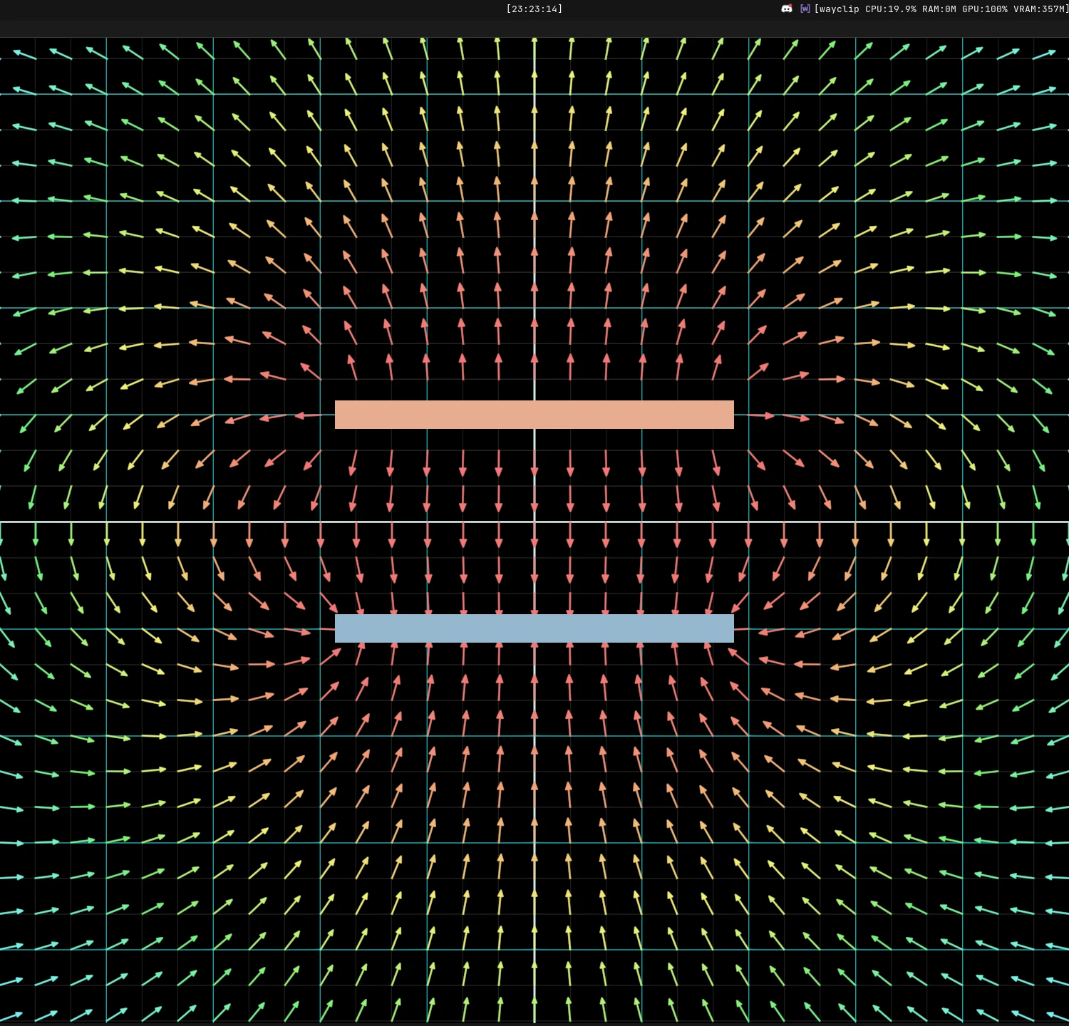
In the end, we were able to try out 2 completely different methods for implementing metal plates: the Jacobi Iterator and the so called Boundary Element Method. The second option resulted in a much more efficient simulation, since it combined both analytic and deterministic results. The result is the ability to create plates that interact with the electric field.

However, the journey does not stop here. As part of this update, I have also reworked the UI/UX experience. Most notebly, in addition to the floating window, a new top bar was added. This top bar gives more information and gives direct access to certain features like tool selection and time management without the hassle of a menu. The tool selection menu was expanded to accomodate: Creation of Charge, Creation of Test Charge, Creation of Metal Plate and the Removal of any element. 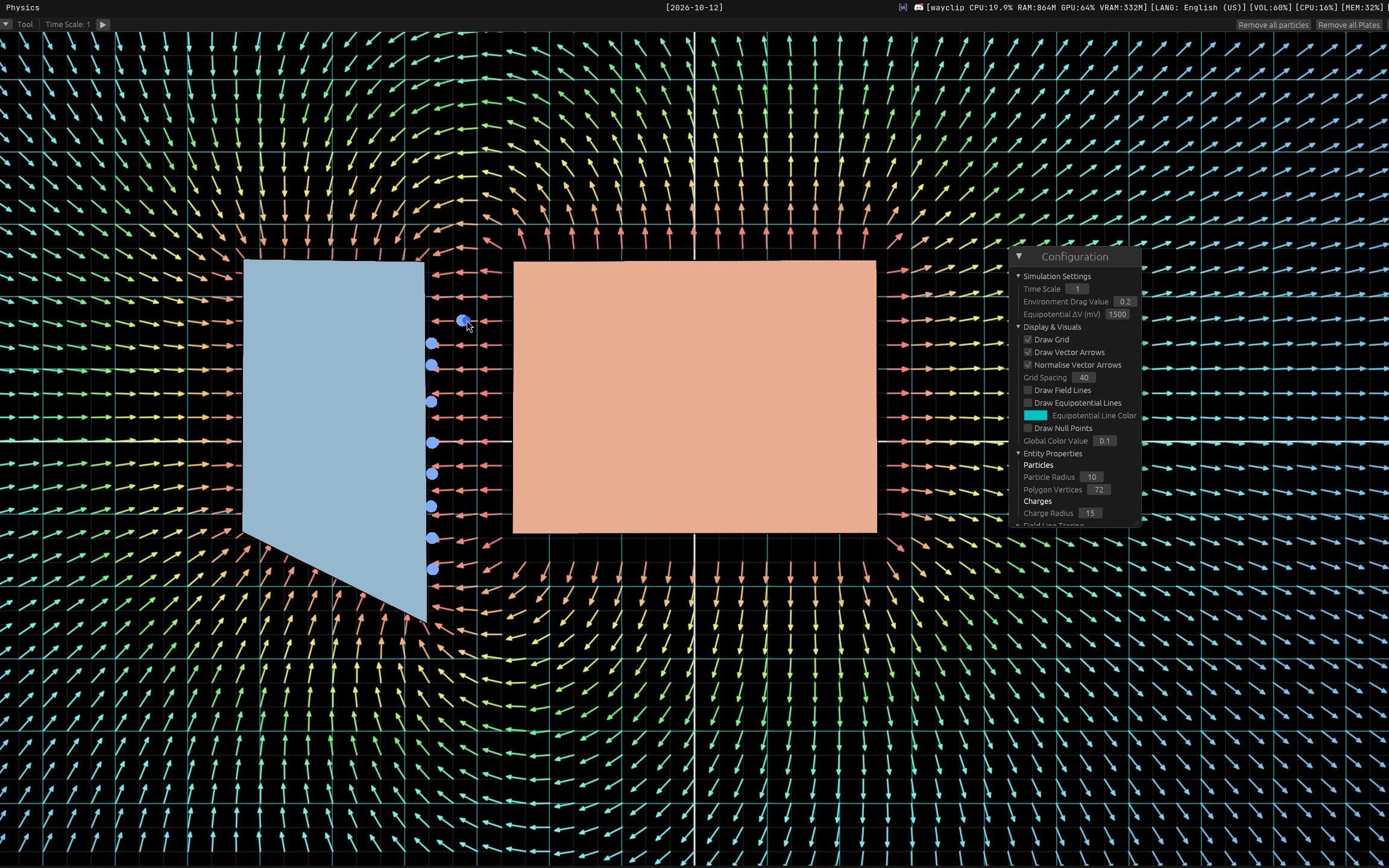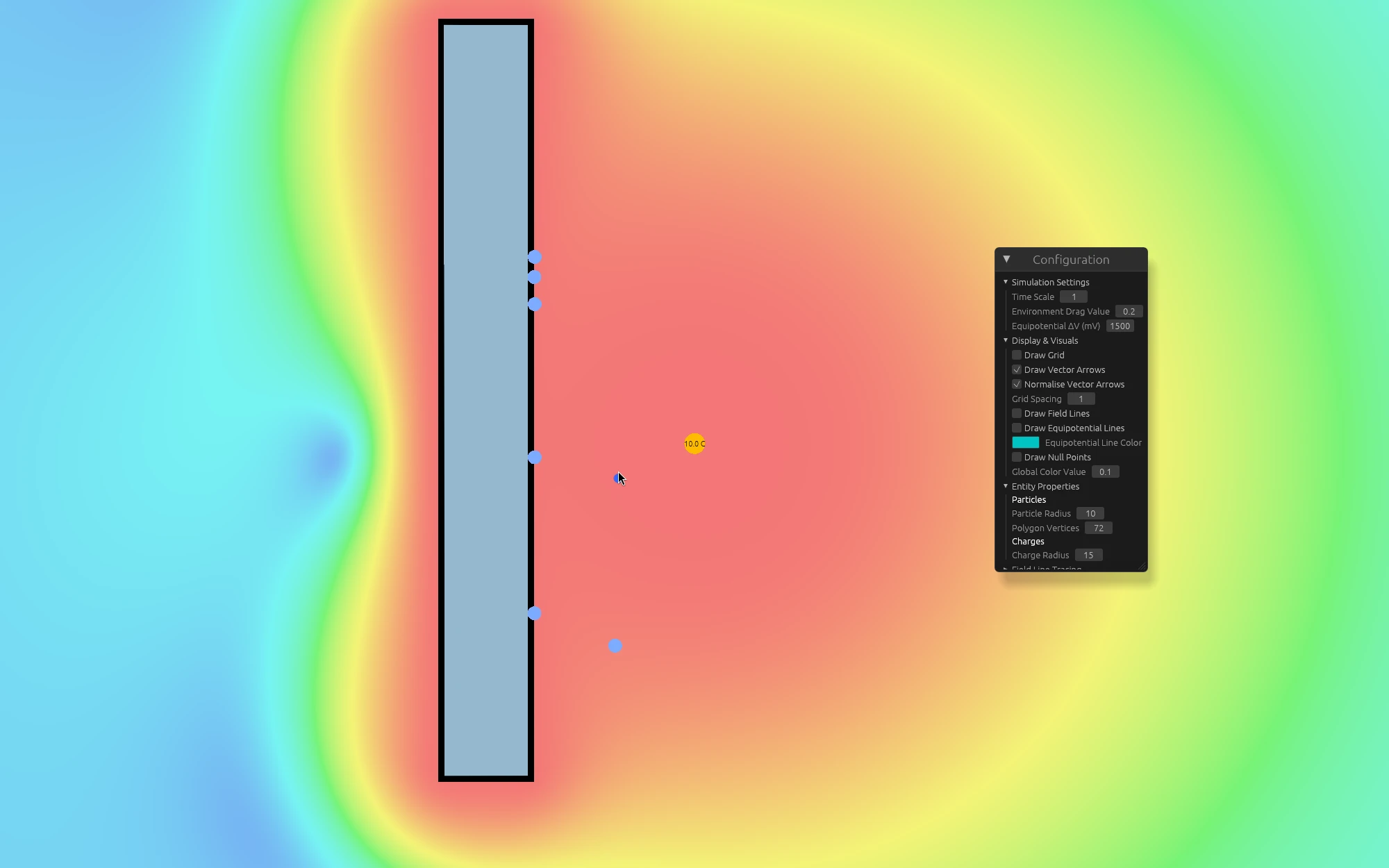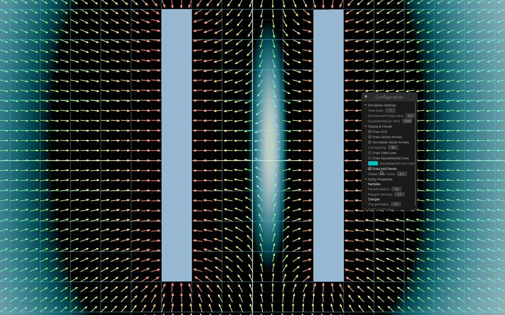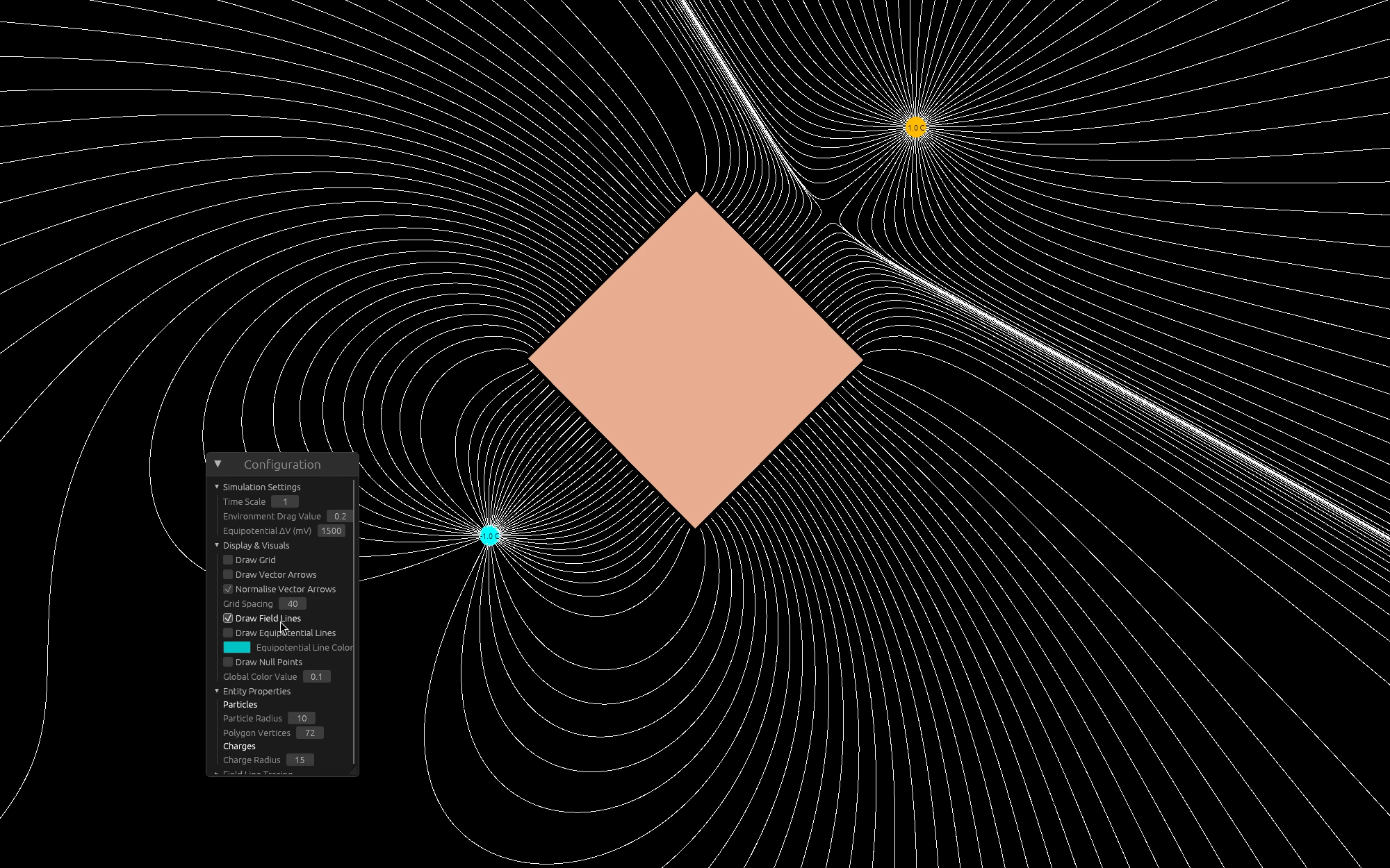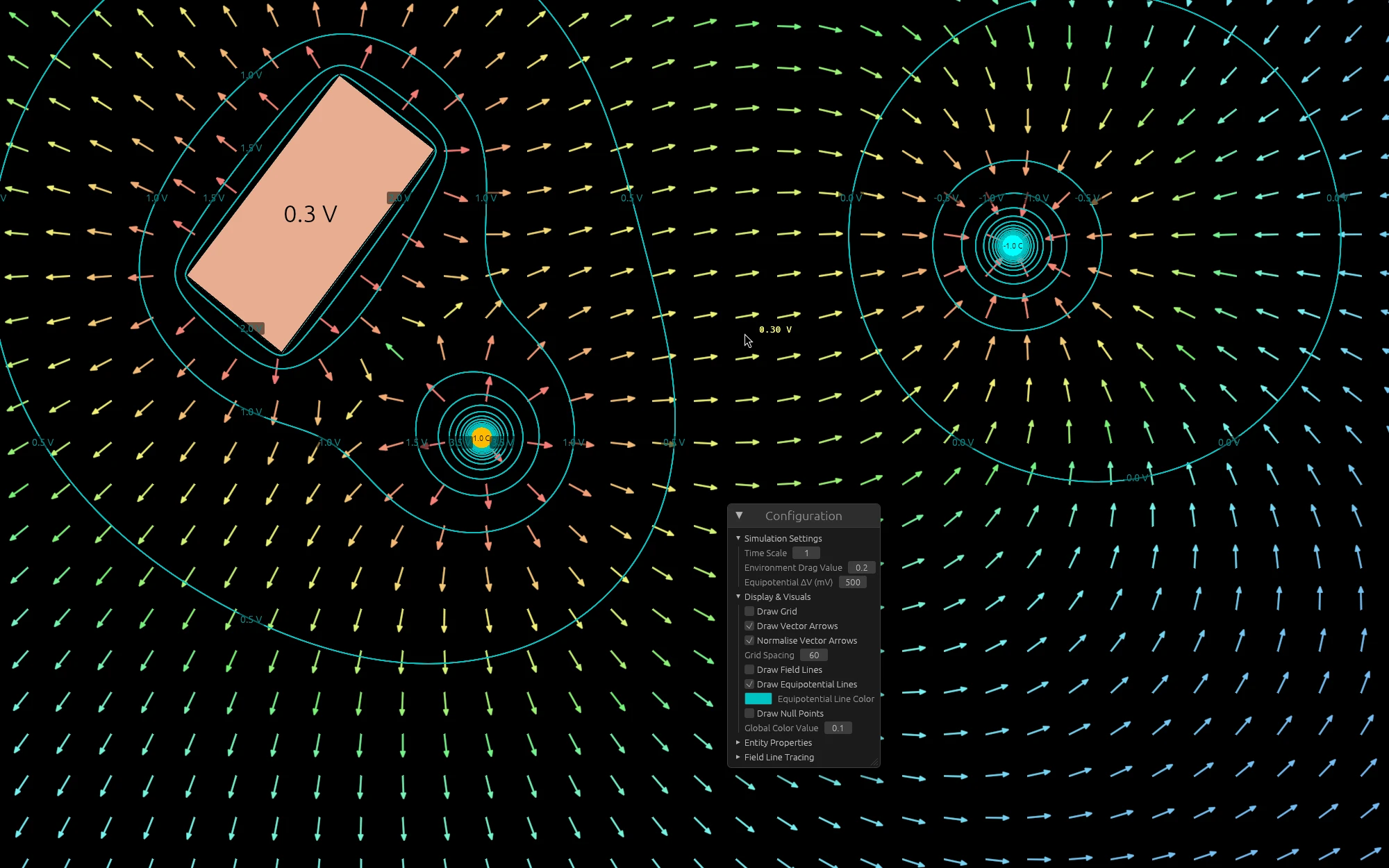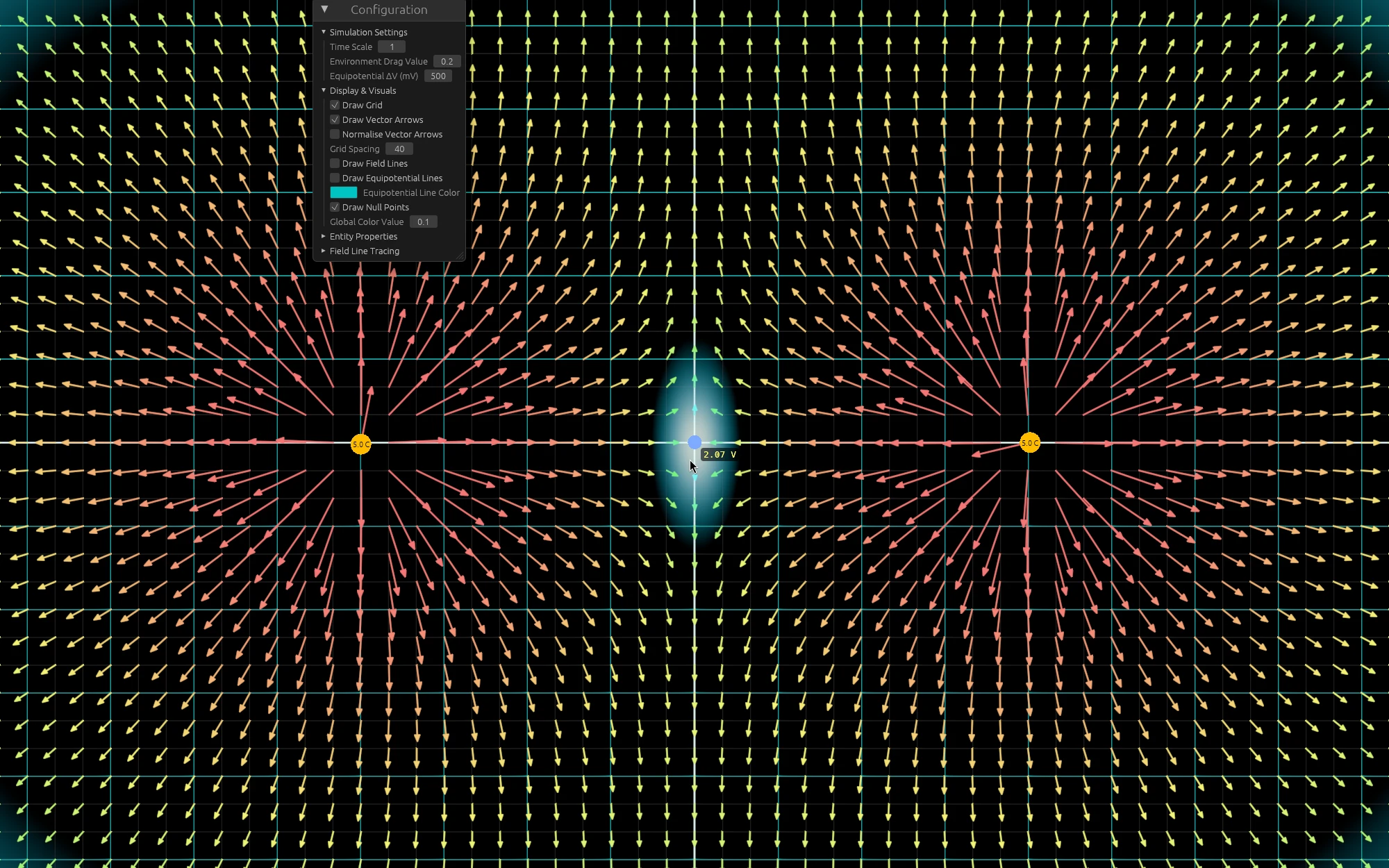The metal plate spawn tool uses a multi-stage setup algorithm, to record the exact points of all 4 vertices, and prompt the user for the Voltage selection. In the end, this gives the freedom to experiment with various systems and designs. The following is a showcase of all the possible configurations possible.

In the future, I want to focus on:

• (a) Optimising, packaging and improving the current simulation to the best of my ability, with features such as presets, multi-threading, and easier controls
• (b) Exploring other areas of electro-magnetism following the Caltech notes (but currently I got really interested in QM via the OCW lectures, so I might do a few topics on that first)

Thank you for reading, and see you all in the next chapter!